22. Riemann Sums, Integrals and the FTC
Riemann sums can be generalized in three ways:
(1) The partitions may not be evenly spaced.
(2) The evaluation points may not be the right endpoints.
(3) The function \(f(x)\) may not be positive.
In that case, the limit of Riemann sums still defines an integral, but the
integral can no longer be interpreted as an area.
If you skip the details on this page, at least read the definition, remark
and proposition in the middle of
this page.
a2. General Riemann Sums and Integrals (Optional)
To find the integral, \(\displaystyle \int_a^b f(x)\,dx\), of the function \(f(x)\) between \(x=a\) and \(x=b\), follow these steps:
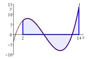
the function is not always positive.
Divide the interval \([a,b]\) into \(n\) subintervals at some partition points: \[ x_0=a< x_1 < x_2 <\cdots < x_{n-1} < x_n=b \] They do not need to be evenly spaced. So, the \(i^\text{th}\) subinterval is \([x_{i-1},x_i]\) and the width of the \(i^\text{th}\) subinterval is \(\Delta x_i=x_i-x_{i-1}\).
It is permissible (but not required) to take all the subintervals to have the same width. In that case, the width of each interval is \( \Delta x=\dfrac{b-a}{n} \) and partition points are \( x_i=a+i\Delta x \) for \( i=0,1,\cdots,n \).
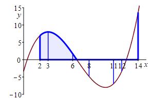
the partition points are: \(2\), \(3\), \(6\), \(8\), \(11\), \(12\), \(14\).
Pick an evaluation point \(x_i^*\) in the \(i^\text{th}\) interval \([x_{i-1},x_i]\). The points can be chosen by some or randomly.
It is permissible (but not required) to take the evaluation point to be the right endpoint of the interval. In that case, \(x_i^*=x_i\).
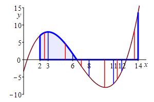
They are randomly located in each interval.
Standard Rules for Riemann Sums
Left Riemann Sum: Evaluate at the left endpoint of each interval.
Right Riemann Sum: Evaluate at the right endpoint of each interval.
Middle Riemann Sum: Evaluate at the midpoint of each interval.
Upper Riemann Sum: Evaluate at the maximum on each interval.
Lower Riemann Sum: Evaluate at the minimum on each interval.
Evaluate the function at the \(i^\text{th}\) evaluation point
and multiply by the width of the \(i^\text{th}\) subinterval to get:
\[
f(x_i^*)\Delta x_i
\]
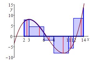
If \(f(x_i^*) \gt 0\), this is the area of the \(i^\text{th}\) rectangle
or an approximation of the area under the curve.
If \(f(x_i^*) \lt 0\), this is the negative of the area of the
\(i^\text{th}\) rectangle or an approximation of the negative of the
area above the curve.
Add these up for all the subintervals to get the
Riemann sum:
\[
\sum_{i=1}^n f(x_i^*)\Delta x_i
\]
which is an approximation to the difference between the area above
the \(x\)-axis and the area below the \(x\)-axis, within the interval
\([a,b]\). The approximation gets better as \(n\) gets larger provided
all subinterval widths, \(\Delta x_i\), approach \(0\).
the value of the function at the evaluation point.
The rectangles above the \(x\)-axis make a
positive contribution to the sum.
The rectangles below the \(x\)-axis make a
negative contribution to the sum.
Take the limit as the number of intervals, \(n\), goes to infinity while also requiring all subinterval widths approach \(0\). This is the definition of an integral as a limit of Riemann sums: \[ \int_a^b f(x)\,dx =\lim_{\begin{aligned}&\scriptstyle\quad n\to\infty \\ &\scriptstyle\text{max}\Delta x_i\to0\end{aligned}} \sum_{i=1}^n f(x_i^*)\Delta x_i \]
If you use equal width intervals and right endpoints, then this formula reduces to \[ \int_a^bf(x)\,dx =\lim_{n\to\infty}\sum_{i=1}^n f(x_i)\Delta x \]
at \(6\) and keeps doubling.
The widths of the intervals are unequal
and the evaluation points are random.
The (definite) integral of a function \(f(x)\) is the limit of the Riemann sums: \[ \int_a^bf(x)\,dx =\lim_{\begin{aligned}&\scriptstyle\quad n\to\infty \\ &\scriptstyle\text{max}\Delta x_i\to0\end{aligned}} \sum_{i=1}^n f(x_i^*)\Delta x_i \]
We can now discuss the implications of the three generalizations of Riemann sums:
- The partitions may not be evenly spaced. However, we can essentially always use partitions with equal spacing. In this course, the only time we will use uneven spacing is to prove the result on Splitting the Interval of an Integral. On the other hand, uneven spacing will become essential in Calculus 3 on Multivariable Calculus.
- The evaluation points may not be the right endpoints. Using other evaluation points is very useful in doing Numerical Integration. An exercise with left endpoints and midpoints is below.
- The function \(f(x)\) may not be positive. In that case the discussion above explains the following result:
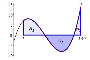
If \(f(x)\) is positive, then the integral \(\displaystyle \int_a^b f(x)\,dx\) gives the area under the graph of \(y=f(x)\) above the \(x\)-axis between \(x=a\) and \(x=b\).
If \(f(x)\) is sometimes positive and sometimes negative, then the integral \(\displaystyle \int_a^b f(x)\,dx\) gives the net area between the graph of \(y=f(x)\) and the \(x\)-axis between \(x=a\) and \(x=b\) with areas above the \(x\)-axis counted positive and areas below the \(x\)-axis counted negative.
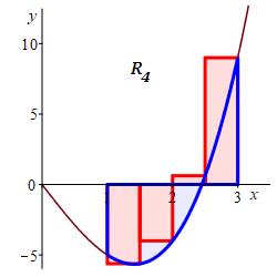
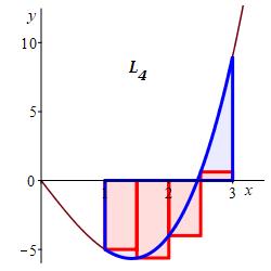
Approximate the integral \(\displaystyle \int_1^3 x^3-6x\,dx\) using a Riemann sum with \(4\) equal width intervals, first using right endpoints and then using left endpoints.
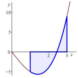
With \(n=4\) intervals, the width is \(\Delta x=\dfrac{3-1}{4}=0.5\).
The right endpoints are: \[ x_1=1.5 \quad x_2=2 \quad x_3=2.5 \quad x_4=3 \] and the function values are: \[\begin{aligned} f(1.5)&=-5.625 & f(2)&=-4 \\ f(2.5)&=0.625 & f(3)&=9 \end{aligned}\] So the Riemann sum is \[\begin{aligned} R_4&=-5.625\cdot0.5-4\cdot0.5 \\ &\quad+0.625\cdot0.5+9\cdot0.5 \\ &=0 \end{aligned}\]
The left endpoints are: \[ x_1=1 \quad x_2=1.5 \quad x_3=2 \quad x_4=2.5 \] and the function values are: \[\begin{aligned} f(1)&=-5 & f(1.5)&=-5.625 \\ f(2)&=4 & f(2.5)&=0.625 \end{aligned}\] So the Riemann sum is \[\begin{aligned} L_4&=-5\cdot0.5-5.625\cdot0.5 \\ &\quad+4\cdot0.5+0.625\cdot0.5 \\ &=-7.0 \end{aligned}\]
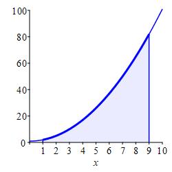
Approximate the integral \(\displaystyle \int_1^9(x^2+1)\,dx\) using:
-
\(4\) equal width subintervals and the left endpoints of each interval.
For equal width intervals \(\Delta x=\dfrac{b-a}{n}\) and for left endpoints \(x_i^*=x_{i-1}\). So: \(\displaystyle \int_a^bf(x)\,dx =\lim_{n\to\infty} \sum_{i=1}^n f(x_{i-1})\Delta x\)
\(L_4=176\)
With \(n=4\) intervals, the width is \(\Delta x=\dfrac{9-1}{4}=2\). For left endpoints, the evaluation points are: \[ x_1=1 \quad x_3=3 \quad x_5=5 \quad x_7=7 \] and the function values are: \[\begin{aligned} f(1)=2\;\, \qquad f(3)=10 \\ f(5)=26 \qquad f(7)=50 \end{aligned}\]
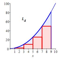
So the Riemann sum is \[ L_4=2(2)+10(2)+26(2)+50(2)=176 \]
-
\(8\) equal width subintervals and the left endpoints of each interval.
\(L_8=212\)
With \(n=8\) intervals, the width is \(\Delta x=\dfrac{9-1}{8}=1\). For left endpoints, the evaluation points are: \[\begin{aligned} x_1&=1 & x_2&=2 & x_3&=3 & x_4&=4 \\ x_5&=5 & x_6&=6 & x_7&=7 & x_8&=8 \end{aligned}\] and the function values are: \[\begin{aligned} f(1)&=2 &\quad f(2)&=5 \\ f(3)&=10 & f(4)&=17 \\ f(5)&=26 & f(6)&=37 \\ f(7)&=50 & f(8)&=65 \end{aligned}\]
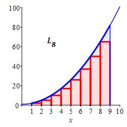
So the Riemann sum is \[ L_8=2+5+10+17+26+37+50+65=212 \]
-
\(4\) equal width subintervals and the midpoints of each interval.
For equal width intervals \(\Delta x=\dfrac{b-a}{n}\) and for midpoints \(x_i^*=\dfrac{x_i+x_{i-1}}{2}\). So: \(\displaystyle \int_a^bf(x)\,dx =\lim_{n\to\infty} \sum_{i=1}^n f(x_i^*)\Delta x\)
\(M_4=248\)
With \(n=4\) intervals, the width is \(\Delta x=\dfrac{9-1}{4}=2\). For midpoints, the evaluation points are: \[ x_2=2 \quad x_4=4 \quad x_6=6 \quad x_8=8 \] and the function values are: \[\begin{aligned} f(2)=5\;\, \qquad f(4)=17 \\ f(6)=37 \qquad f(8)=65 \end{aligned}\]
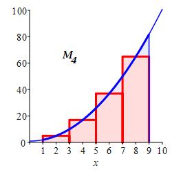
So the Riemann sum is \[ M_4=5(2)+17(2)+37(2)+65(2)=248 \]
-
\(8\) equal width subintervals and the midpoints of each interval.
\(M_8=250\)
With \(n=8\) intervals, the width is \(\Delta x=\dfrac{9-1}{8}=1\). For midpoints, the evaluation points are: \[\begin{aligned} x_1&=1.5 & x_2&=2.5 & x_3&=3.5 & x_4&=4.5 \\ x_5&=5.5 & x_6&=6.5 & x_7&=7.5 & x_8&=8.5 \end{aligned}\] The function is \(f(x)=x^2+1\) and the function values are: \[\begin{aligned} f(1.5)&=3.25 & f(2.5)&=7.25 \\ f(3.5)&=13.25 & f(4.5)&=21.25 \\ f(5.5)&=31.25 & f(6.5)&=43.25 \\ f(7.5)&=57.25 & f(8.5)&=73.25 \end{aligned}\]
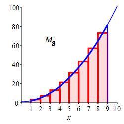
So the Riemann sum is \[\begin{aligned} M_8&=3.25+7.25+13.25+21.25 \\ &\quad+31.25+43.25+57.25+73.25 \\ &=250 \end{aligned}\]
Here is a summary of the left, middle and right Riemann sum approximations to the integral \(\displaystyle \int_1^9(x^2+1)\,dx\) as found in this exercise and in the exercise on the previous page: \[\begin{aligned} &\text{left} &L_4&=176 &L_8&=212 \\ &\text{middle} &M_4&=248 &M_8&=250 \\ &\text{right} &R_4&=336 &R_8&=292 \end{aligned}\] The actual integral is \(\displaystyle \int_1^9(x^2+1)\,dx=\dfrac{752}{3}\approx250.67\) as found in an exercise on the next page. Clearly, more intervals give a better approximation.
Since the function \(f(x)=x^2+1\) is increasing, the plots explain why the left sums give lower bounds (under estimates), the right sums give upper bounds (over estimates) and the middle sums give better estimates. This is a case of Mama Bear, Papa Bear and Baby Bear.
See the chapter on Numerical Integration in Calculus 2 for more details about Riemann sums and other approximations for integrals.


In practice, one does not compute integrals using the Riemann sum formula. Rather, one uses this formula to derive the integral that needs to be computed in various applications (such as area). The integral is then computed using antiderivatives as prescribed by the Fundamental Theorem of Calculus: \[ \int_a^bf(x)\,dx=F(b)-F(a) \] as discussed on the page after next. However, we first discuss how the limits of Riemann sums are computed in simple cases on the next page.
Heading
Placeholder text: Lorem ipsum Lorem ipsum Lorem ipsum Lorem ipsum Lorem ipsum Lorem ipsum Lorem ipsum Lorem ipsum Lorem ipsum Lorem ipsum Lorem ipsum Lorem ipsum Lorem ipsum Lorem ipsum Lorem ipsum Lorem ipsum Lorem ipsum Lorem ipsum Lorem ipsum Lorem ipsum Lorem ipsum Lorem ipsum Lorem ipsum Lorem ipsum Lorem ipsum